A smoother waveform does not automatically mean a more accurate measurement. When estimating pulse wave velocity (PWV), a processing choice can influence the result even before any biological interpretation begins.
The timing behind PWV
PWV is calculated as distance divided by pulse transit time. Our 2023 study examined how the interpolation time step affects transit-time estimation using cross-correlation of 4D flow MRI waveforms.
Testing the processing choice
Experiments used flexible and stiff phantoms with varying flow and beat frequency. A critical interpolation time step was selected to balance differences in estimated PWV against computation time. In vivo comparisons included six healthy volunteers.
What changed?
In the in vitro Bland–Altman analysis, the mean difference against the 0.1 ms numerical reference was 0.730 m/s with the conventional 1 ms step and 0.140 m/s with the optimized step. These are differences from a numerical reference, not estimates of clinical diagnostic accuracy. Volunteer estimates were similar between the optimized and conventional approaches.
The reference matters
The in vitro reference was PWV calculated using a 0.1 ms interpolation step. Thus, the reported improvement concerns agreement with a finer numerical reference, not an independent invasive measurement. Interpolation also cannot recover temporal information that the scan never acquired.
A useful reporting habit
For any derived measurement, readers benefit from knowing both the acquisition and processing settings. A comparison becomes easier to assess when the report names the algorithm, time step, distance definition, and reference used.
For broader context, compare PWV reference values by age and measurement method and read about structural and load-dependent arterial stiffness.
Why a millisecond can matter
Consider an illustrative example, not a participant result: a pulse traveling 0.10 m in 20 ms gives a PWV of 5.0 m/s. A transit-time estimate of 19 ms gives 5.26 m/s, while 21 ms gives 4.76 m/s. A small timing difference can therefore change the reported speed even when the path length is identical.
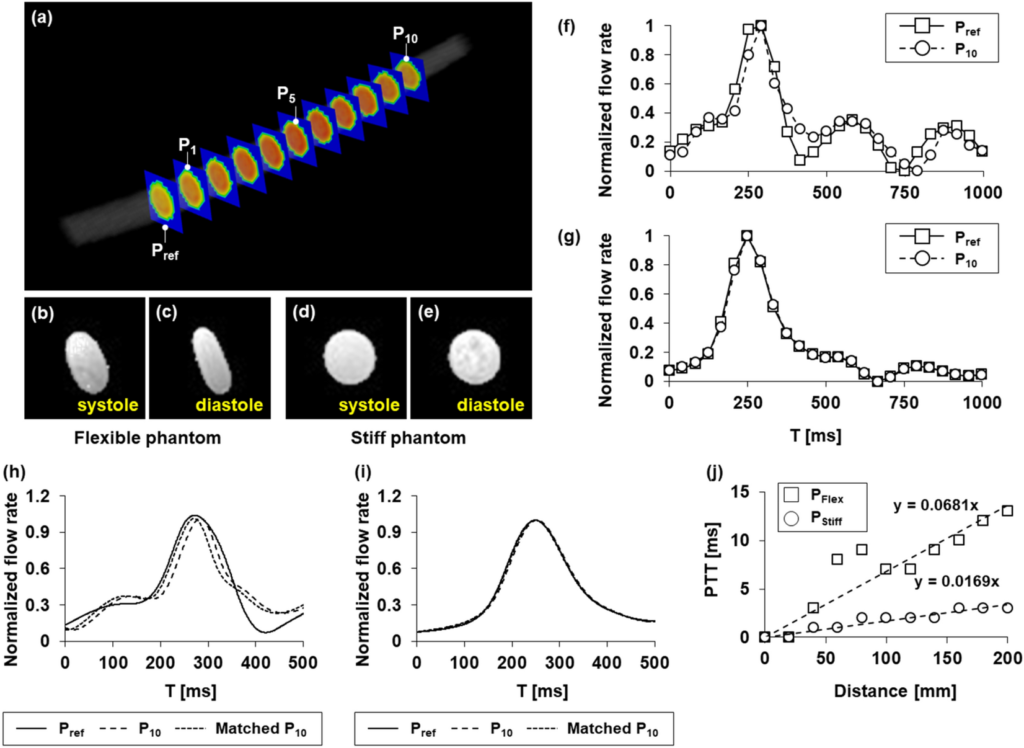
Cross-correlation estimates the shift that best aligns two flow waveforms. Interpolation changes the time grid used to search for that shift. It can refine the numerical estimate, but it does not create new acquired MRI frames or replace adequate image quality. Figure 3 illustrates this alignment using the flexible and stiff phantom waveforms.
When comparing studies, match the arterial segment and analysis method before interpreting different PWV values. For reproducible reporting, describe the path-length definition, waveform sampling, interpolation step, and transit-time algorithm alongside the final speed.
Flexible versus stiff: following the pulse in Figure 3
The flexible and stiff phantoms make the timing problem visible. At the illustrated flow and beat-frequency condition, the flexible model’s distal waveform was delayed relative to the reference waveform, whereas the stiff model’s waveforms were much closer in time. The figure then shows how cross-correlation aligns the waveforms and how transit time changes with measurement distance.
This controlled comparison separates a processing question from the complexity of human anatomy. When the measured delay is short, a fixed interpolation step occupies a larger fraction of that delay. That explains why the same numerical setting can behave differently across the two models.
Original paper
Park S, Kwon M, Nam H, Huh H. Interpolation time-optimized aortic pulse wave velocity estimation by 4D flow MRI. Scientific Reports. 2023;13:16484. Read the paper.
Keywords: 4D flow MRI PWV, pulse transit time, waveform interpolation, cross-correlation, temporal resolution, aortic stiffness.